

How Do You Filter In A Plot In R
Decomposing South African output
The commencement program for this session contains diverse filters that may be used to decompose a measure of South African output. This example is contained in the file T5-decomp.R. Once over again, the first thing that we practice is articulate all variables from the current environment and close all the plots. This is performed with the following commands:
rm(list = ls()) graphics.off() Thereafter, nosotros will need to install the tsm package from my GitHub business relationship, as well as the mFilter package that was written by one of my co-authors.
devtools:: install_github("KevinKotze/tsm") install.packages("mFilter", repos = "https://cran.rstudio.com/", dependencies = Truthful) The next stride is to make sure that yous can access the routines in these packages by making use of the library control.
library(tsm) library(mFilter) Load the data
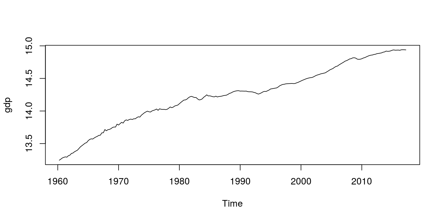
Equally noted previosuly, South African GDP data has been preloaded in the tsm bundle, where Real GDP is numbered KBP6006D. Hence, to retrieve the information from the package and create the object for the natural logarithm of GDP that volition exist stored every bit a time series in gdp, we execute the following commands:
dat <- sarb_quarter$KBP6006D dat.tmp <- log(na.omit(dat)) gdp <- ts(dat.tmp, start = c(1960, 2), frequency = 4) To make sure that these calculations and extractions take been performed correctly, we audit a plot of the information.
Detrend information with a linear filter
To estimate a linear tendency nosotros can make utilise of a linear regression model that includes a time trend and a abiding. To gauge such a model nosotros make apply of the lm command as follows.
lin.modernistic <- lm(gross domestic product ~ time(gdp)) lin.trend <- lin.modernistic$fitted.values # fitted values pertain to time tendency linear <- ts(lin.trend, start = c(1960, 1), frequency = 4) # create a time series variable for tendency lin.cycle <- gdp - linear # wheel is the divergence betwixt the data and linear tendency The fitted values from the regression would and so comprise the information that pertains to the linear tendency. These would demand to exist extracted from the model object lin.mod and in the above chunk we take allocated these values to the fourth dimension series object linear. The cycle is so derived from subtracting the trend from the data.
Nosotros can then plot this event with the assistance of the post-obit commands, where the tendency and the bike are plotted on separate figures.
par(mfrow = c(1, 2), mar = c(2.two, two.2, 1, 1), cex = 0.8) # plot two graphs adjacent and squash margins plot.ts(gdp, ylab = "") # first plot fourth dimension series lines(linear, col = "red") # include lines over the plot legend("topleft", legend = c("data", "tendency"), lty = 1, col = c("black", "red"), bty = "n") plot.ts(lin.cycle, ylab = "") # 2nd plot for cycle legend("topright", legend = c("cycle "), lty = 1, col = c("black"), bty = "north") 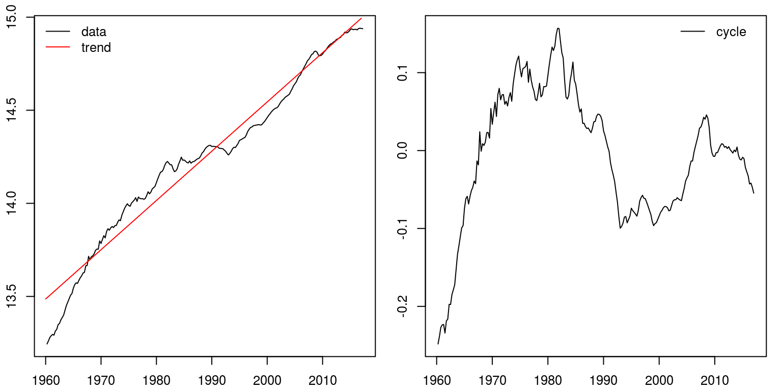
Detrend data with the Hodrick-Prescott filter
To detrend this data with the popular Hodrick-Prescott filter we only need to brand use of a unmarried command. In this case we are setting the value for lambda equal to 1600, which is what has been suggested for quarterly data.
hp.decom <- hpfilter(gdp, freq = 1600, blazon = "lambda") par(mfrow = c(1, 2), mar = c(2.two, two.2, 1, one), cex = 0.8) plot.ts(gdp, ylab = "") # plot time series lines(hp.decom$trend, col = "red") # include HP trend fable("topleft", legend = c("data", "HPtrend"), lty = 1, col = c("black", "red"), bty = "n") plot.ts(hp.decom$cycle, ylab = "") # plot bike legend("topleft", fable = c("HPcycle"), lty = i, col = c("black"), bty = "north") 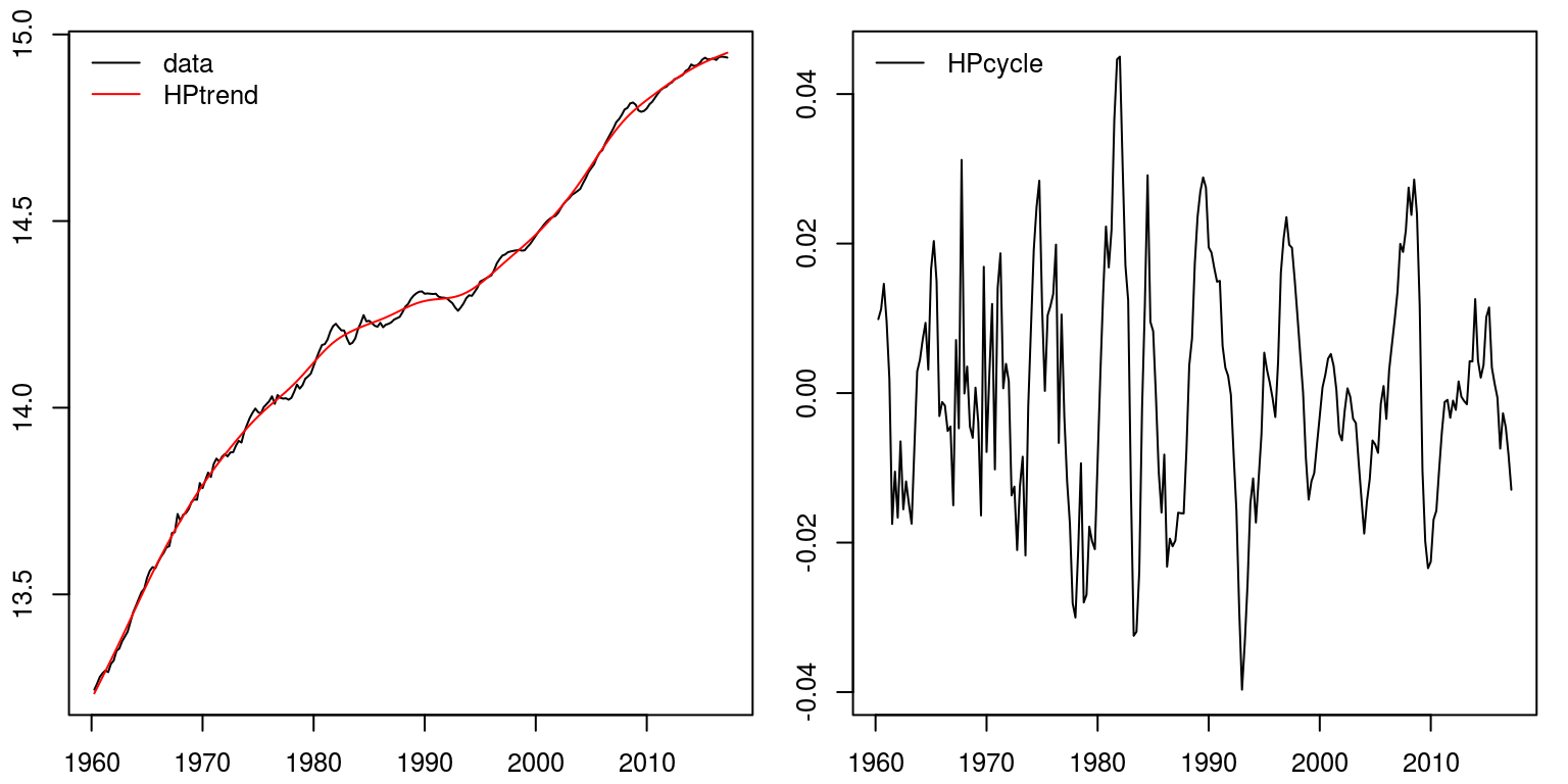
Annotation that this would announced to provide a more accurate representation of what we empathise of South Africas economic functioning.
Detrend information with the Baxter-King filter
To make use of the Baxter-King band pass filter we can employ a similar command to what was used above. In this case we need to specify the frequency band for the cycle, where the upper limit is prepare at 32 and lower limit is set up at 6.
bp.decom <- bkfilter(gdp, pl = 6, pu = 32) par(mfrow = c(ane, 2), mar = c(2.two, two.2, ane, one), cex = 0.8) plot.ts(gdp, ylab = "") lines(bp.decom$trend, col = "red") legend("topleft", legend = c("data", "BPtrend"), lty = 1, col = c("blackness", "red"), bty = "northward") plot.ts(bp.decom$cycle, ylab = "") legend("topleft", legend = c("BPcycle"), lty = ane, col = c("black"), bty = "due north") 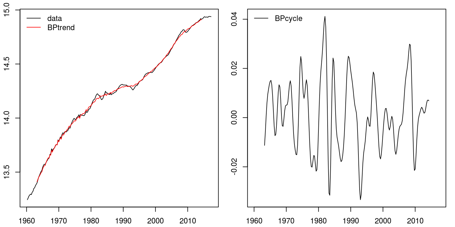
Once again this seems to provide a fairly accurate representation of the cyclical nature of economic activity in Southward Africa. Note also that the representation of the bicycle is much smoother than what was provided previously, as the racket is not included with the cycle.
Detrend data with the Christiano-Fitzgerald filter
This filter is very similar in nature to what was provided above. In addition, information technology also generates a highly similar event to that of the Baxter-King filter.
cf.decom <- cffilter(gdp, pl = six, pu = 32, root = Truthful) par(mfrow = c(one, ii), mar = c(2.two, 2.2, 1, 1), cex = 0.eight) plot.ts(gdp, ylab = "") lines(cf.decom$trend, col = "red") legend("topleft", legend = c("data", "CFtrend"), lty = 1, col = c("black", "red"), bty = "due north") plot.ts(cf.decom$bike, ylab = "") legend("topleft", legend = c("CFcycle"), lty = one, col = c("black"), bty = "n") 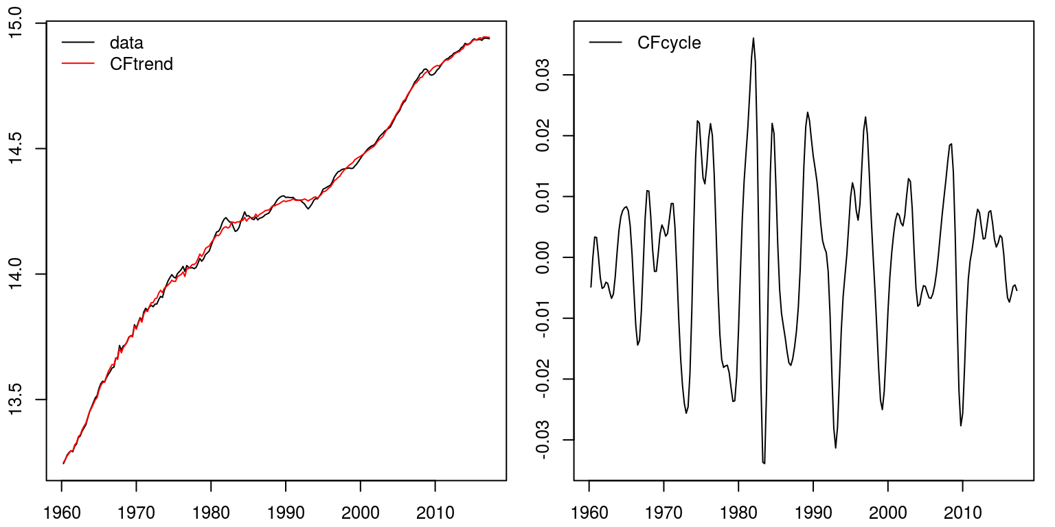
Detrend data with the Beveridge-Nelson decomposition
To decompose output into a stochastic trend and stationary cycle, we can employ the Beveridge-Nelson decomposition. When employing this technique we would need to specify the number of lags that would pertain to the stationary component. In the example that I've included below, I've assume eight lags.
bn.decomp <- bnd(gross domestic product, nlag = eight) # apply the BN decomposition that creates dataframe bn.trend <- ts(bn.decomp[, 1], commencement = c(1960, 1), frequency = iv) # first column contains trend bn.cycle <- ts(bn.decomp[, 2], get-go = c(1960, 1), frequency = 4) # 2d column contains cycle par(mfrow = c(1, ii), mar = c(2.2, 2.2, 1, one), cex = 0.8) plot.ts(gross domestic product, ylab = "") lines(bn.tendency, col = "blood-red") fable("topleft", legend = c("data", "BNtrend"), lty = i, col = c("black", "ruby"), bty = "north") plot.ts(bn.bike, ylab = "") fable("topleft", legend = c("BNcycle"), lty = 1, col = c("black"), bty = "n") 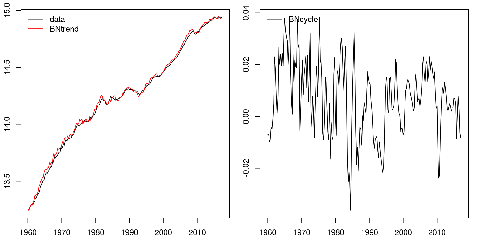 ## Comparison different measures of the cycle
We can then combine all these results on a single graph to consider the respective similarities and differences. In this instance, I've created a time series wedlock, ts.marriage, but I could have besides plotted a single serial, before using the lines control to plot successive plots on peak of that.
comb <- ts.spousal relationship(lin.cycle, hp.decom$cycle, bp.decom$bicycle, cf.decom$cycle, bn.cycle) par(mfrow = c(1, 1), mar = c(2.2, 2.2, 2, 1), cex = 0.viii) plot.ts(comb, ylab = "", plot.type = "unmarried", col = c("blueish", "ruddy", "darkgrey", "sienna", "darkgreen")) legend("topleft", legend = c("linear", "hp-filter", "bp-filter", "cf-filter", "bn-decomp"), lty = 1, col = c("blue", "red", "darkgrey", "sienna", "darkgreen"), bty = "north") 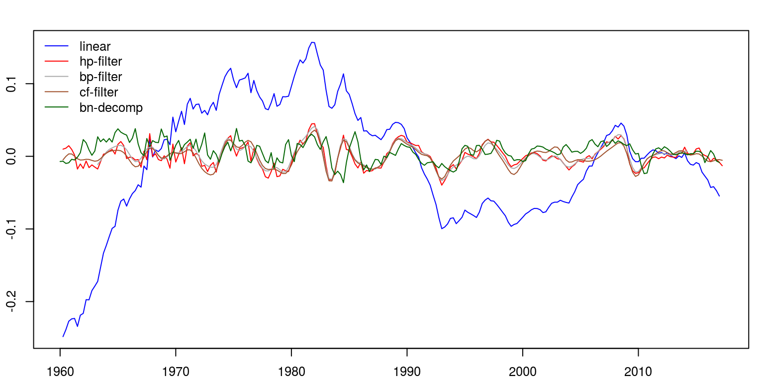
Spectral decompositions
Before we consider the use of spectral techniques it would be a good idea to articulate all variables from the current environment and close all the plots.
rm(list = ls()) graphics.off() The next step is to make sure that you can access the routines in these packages by making use of the library command.
library(tsm) library(TSA) library(mFilter) In class we simulated some data and decomposed it using spectral techniques. To replicate this case, we could generate values for three time series variables, which are then combined to form a unmarried variable.
no.obs <- 100 t <- seq(1, no.obs, one) w <- c(6 /no.obs, 30 /no.obs, twoscore /no.obs) x1 <- 2 * cos(2 * pi * t * w[1]) + 3 * sin(two * pi * t * w[1]) # frequency six cycles in no.obs points x2 <- 4 * cos(2 * pi * t * west[2]) + 5 * sin(2 * pi * t * w[2]) # frequency ten cycles in no.obs points x3 <- half dozen * cos(2 * pi * t * west[3]) + 7 * sin(2 * pi * t * w[3]) # frequency xl cycles in no.obs points y <- x1 + x2 + x3 To expect at the behaviour of these variables we can plot them on a separate axes.
par(mfrow = c(2, 2), mar = c(2.2, 2.2, 2, 1), cex = 0.eight) plot(x1, type = "50", main = "x1") plot(x2, type = "fifty", principal = "x2") plot(x3, blazon = "fifty", main = "x3") plot(y, type = "l", main = "y") 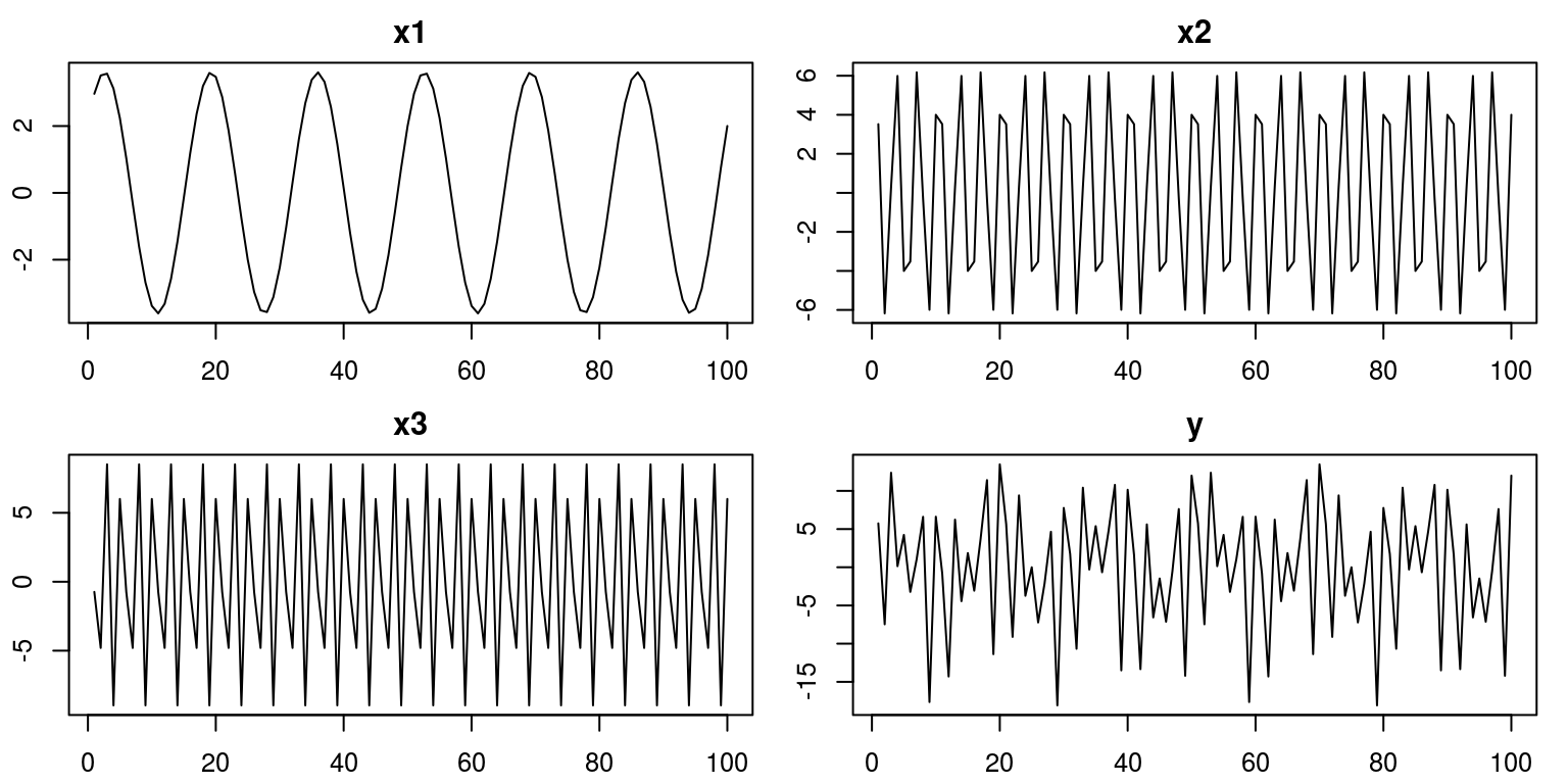
Thereafter, we could utilize the periodogram to consider the properties of each of these fourth dimension series variables.
periodogram(x1, chief = "x1", col = "red") 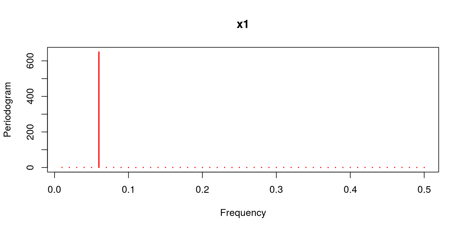
periodogram(x2, master = "x2", col = "red") 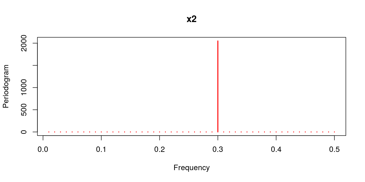
periodogram(x3, main = "x3", col = "red") 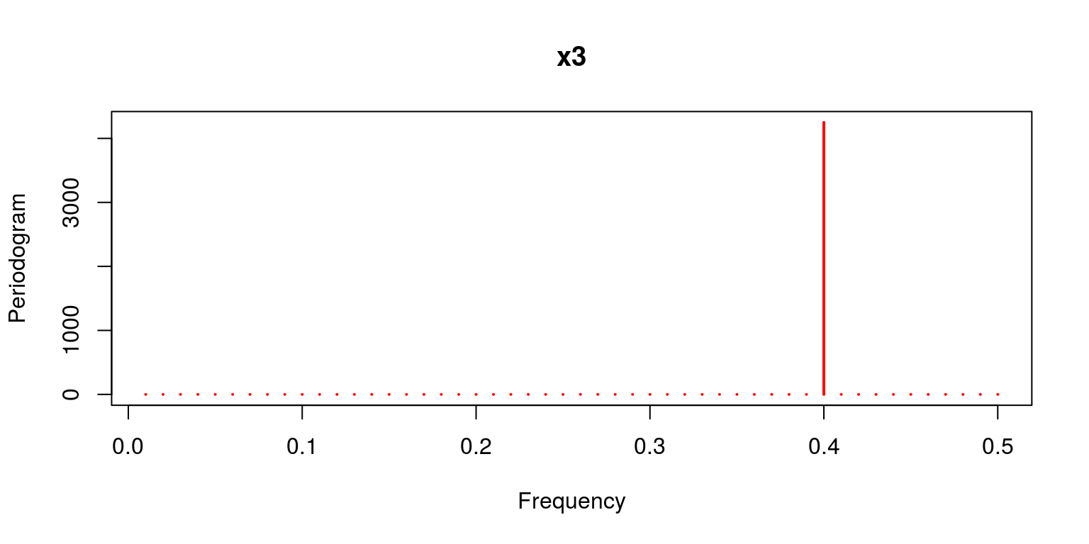
periodogram(y, master = "y", col = "red") 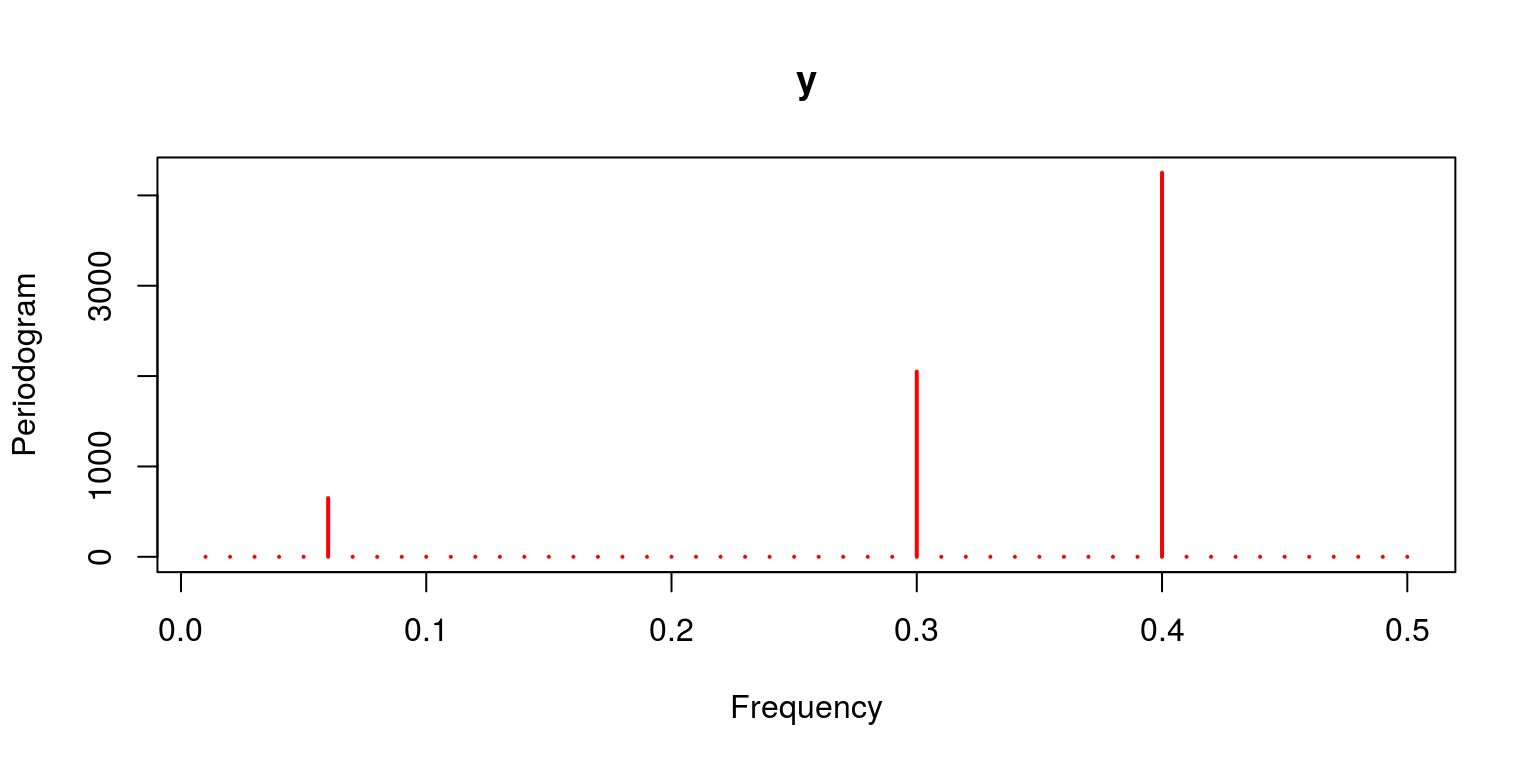
We could of course make use of a filter to remove some of the unwanted components from the aggregate time series variable. To do so we could apply the Christiano-Fitzgerald filter with a relatively narrow upper and lower bound. Thereafter we utilize the periodogram that is applied to information relating to the cycle, to investigate whether it successfully excluded some of the frequency components.
ybp <- cffilter(y, pl = 16, pu = 20) par(mfrow = c(one, 1)) periodogram(ybp$cycle, col = "cherry") 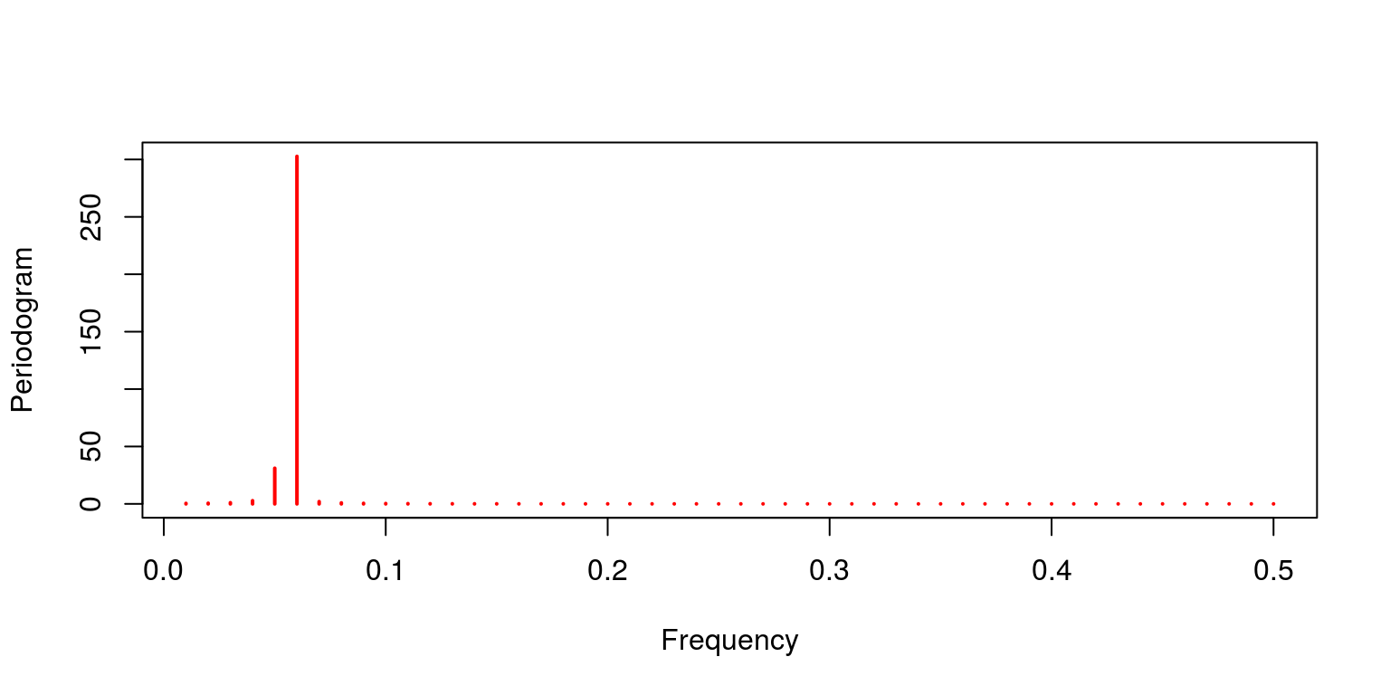
This issue would propose that the filter has excluded most of the higher frequency components. To see how this cycle relates to the previous data we plot the cyclical data that passed through the filter onto the slow moving component. In addition, we likewise plot this issue on the variable for the combined cycles.
par(mfrow = c(one, 2), mar = c(2.2, 2.2, 2, ane), cex = 0.8) plot(x1, type = "fifty", lty = i) lines(ybp$bicycle, lty = 3, lwd = iii, col = "cherry") legend("topleft", fable = c("X1", "Filtered "), lty = c(1, three), col = c("blackness", "red"), bty = "n") plot(y, blazon = "50", lty = 1) lines(ybp$bicycle, lty = 3, lwd = 3, col = "ruby") legend("topleft", legend = c("Actual", "Filtered "), lty = c(1, 3), col = c("blackness", "red"), bty = "n") 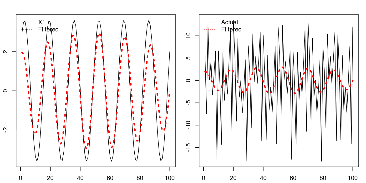
In both cases it would appear to do a reasonable chore of characterising the trend in the process.
Spectral decompositions on the South African business cycle
To consider how these spectral decompositions may be used in practice we tin now consider the use of these techniques when practical to various characterisations of the South African business organization cycle. It would be useful to beginning this application with a make clean workspace and plot window.
rm(list = ls()) graphics.off() The next step would exist to run all the filters that were applied to place the different measures of the Due south African business bike. Hence, to run the previous program we tin use the source command, where we include the proper noun of the file.
Allow us at present apply a periodogram to each measure of the business organization cycle.
periodogram(lin.cycle, main = "Linear", col = "cerise") 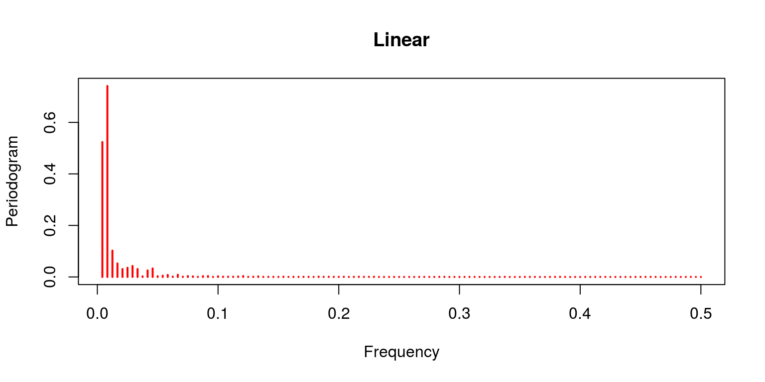
periodogram(hp.decom$bike, main = "Hodrick-Prescott", col = "cerise") 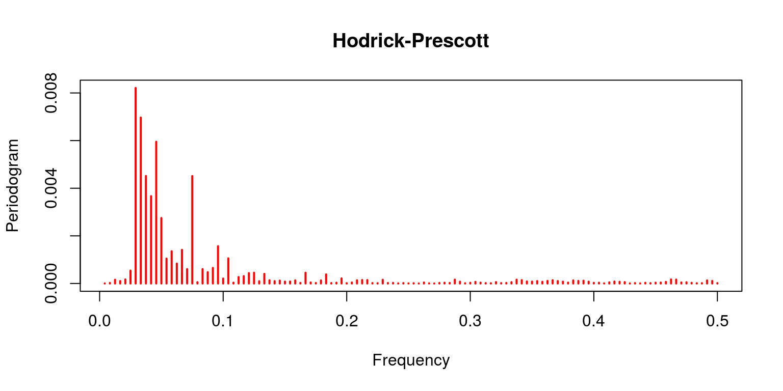
periodogram(bp.decom$bike[13 :(length(bp.decom$bike) - 12)], chief = "Band-Pass", col = "red") 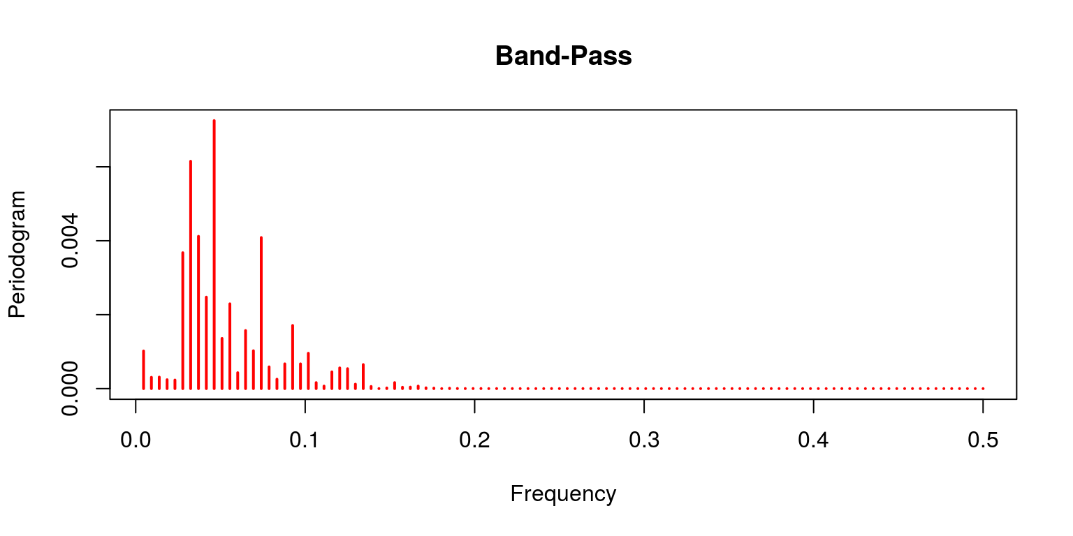
periodogram(cf.decom$bike, primary = "Christiano-Fitzgerald", col = "red") 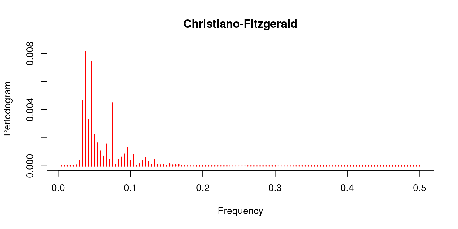
periodogram(bn.cycle, main = "Beveridge-Nelson", col = "red") 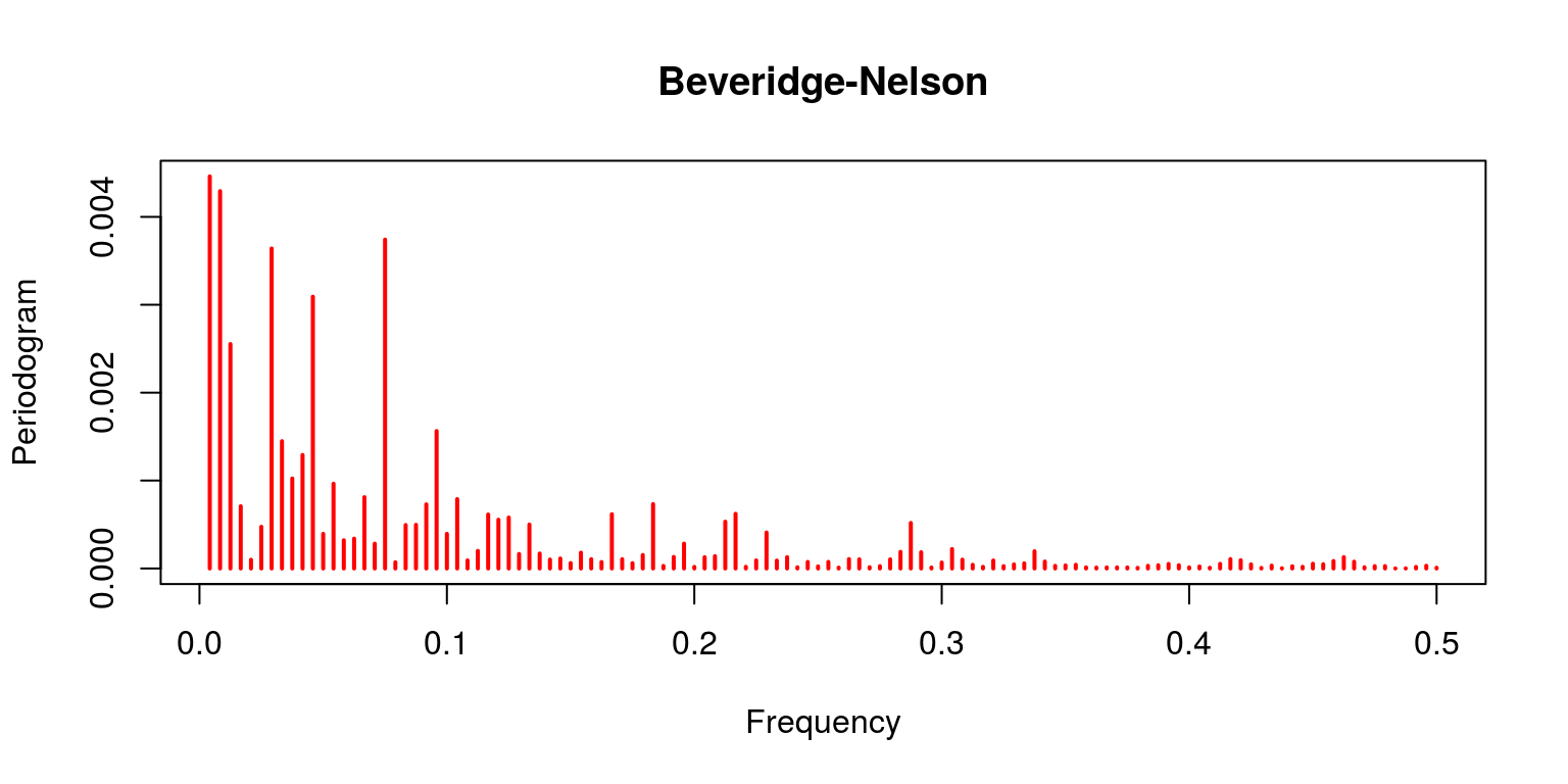
Notation that the linear filter provides a poor effect as the trend clearly dominates (which is not what should be expected of the cycle). This is contrast with the characterisation of the Hodrick-Prescott filter, where the trending data has been removed. This is also the case for both the Band-Pass filters of Baxter & King and Christiano & Fitzgerald. In both of these cases the noise has as well been removed. The final result pertains to the Beveridge-Nelson decomposition, where we notation that the cycle includes a great deal of the trend and a large element of noise.
Wavelet decompositions
To provide an example of the wavelet decomposition nosotros will apply the technique to data for South African aggrandizement. This would allow use to derive an culling measure for trend in the process, which may be considered to correspond core inflation. Note that this technique may be applied to data of any integration social club so nosotros do not need to firstly consider the integration club of the variables. Again, it would be useful to start with a clean workspace and plot window.
rm(listing = ls()) graphics.off() In this case nosotros will brand utilize of the waveslim and tsm packages.
library(tsm) library(waveslim) We will then make of monthly data for the consumer price index, which is contained the SARB quarterly bulletin release. The numeric for this variable is KBP7170N and the data extends back to 2002. To calculate a year-on-year measure of aggrandizement nosotros then make apply of the diff and lag commands.
dat <- sarb_month$KBP7170N cpi <- ts(na.omit(dat), start = c(2002, 1), frequency = 12) inf.yoy <- diff(cpi, lag = 12)/cpi[- 1 * (length(cpi) - 11): length(cpi)] To ensure that all these variable transformations accept been performed correctly we plot the information.
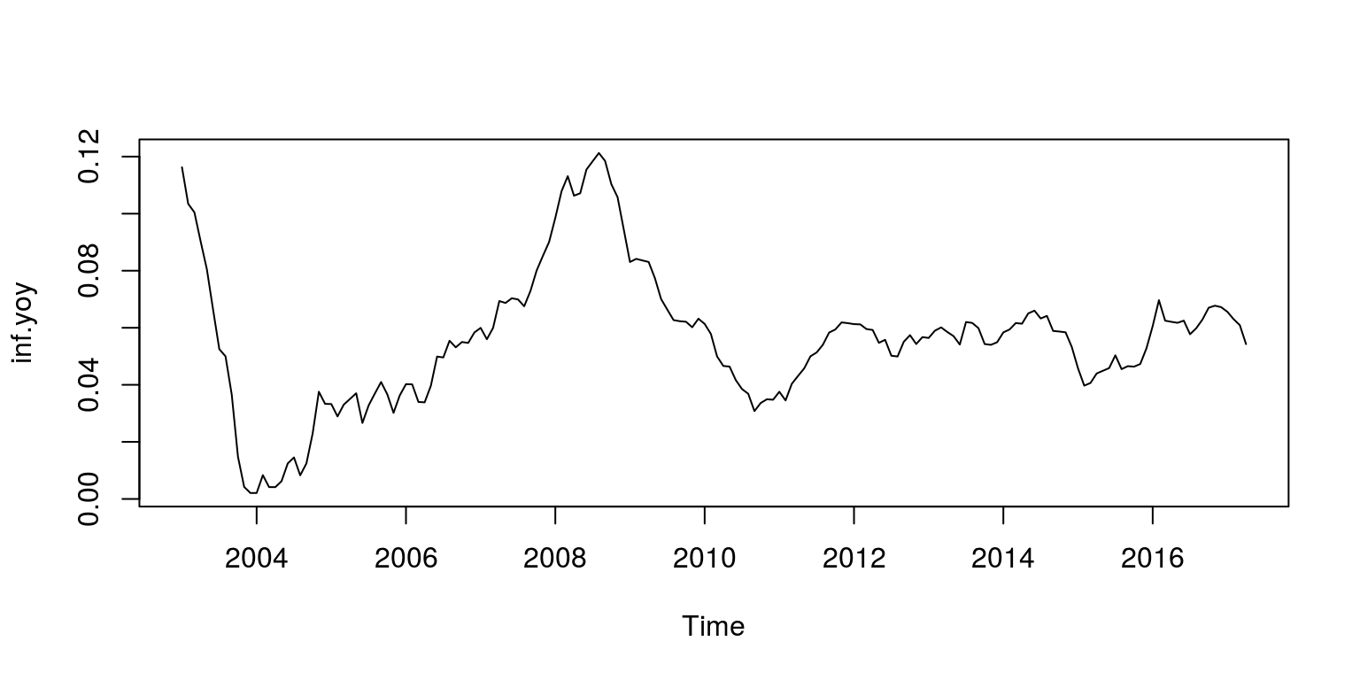
As we are primarily interested in identifying the smoothed trend in this case, nosotros will make use of a Daubechies function that is neither too smooth or sharp. Such a part would exist the Daubechies 4 wavelet, that will be applied with the aid of the modified discrete wavelet transformation technqiue. In add-on, we are also going to brand apply of iii mother wavelets for the respective high frequency components.
inf.d4 <- modwt(inf.yoy, "d4", north.levels = three) names(inf.d4) <- c("w1", "w2", "w3", "v3") inf.d4 <- stage.shift(inf.d4, "d4") Nosotros can then plot the results for each of the separate frequency components as follows:
par(mfrow = c(five, i)) plot.ts(inf.yoy, axes = FALSE, ylab = "actual", principal = "") for (i in i : 4) { plot.ts(inf.d4[[i]], axes = Simulated, ylab = names(inf.d4)[i]) } axis(side = i, at = c(seq(i, (length(inf.yoy)), by = 48)), labels = c("2002", "2006", "2010", "2014")) 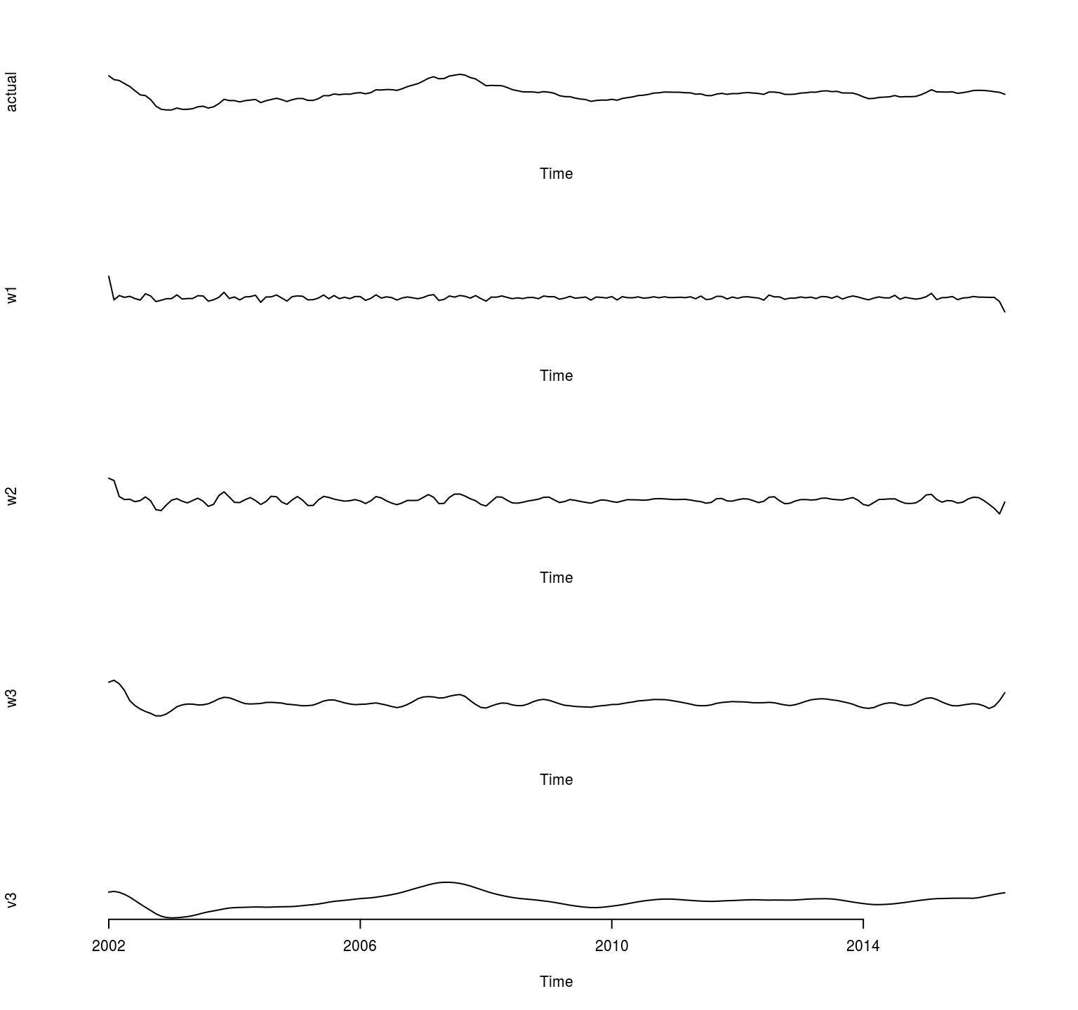
If we now want to plot the trend (father wavelet) on the data.
inf.tren <- ts(inf.d4$v3, start = c(2003, i), frequency = 12) plot.ts(inf.yoy, ylab = "inf") lines(inf.tren, col = "red") 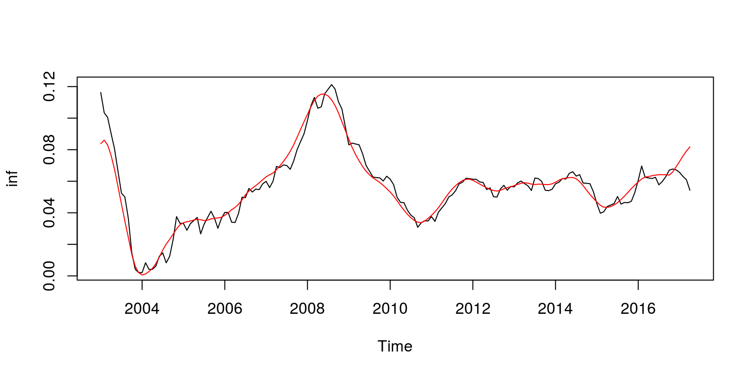
Annotation that equally the corresponding scales (or frequency bands) are additive, we could add ane of the mother frequency bands to the tendency as follows.
inf.tmp <- inf.tren + inf.d4$w3 inf.tren2 <- ts(inf.tmp, kickoff = c(2003, one), frequency = 12) plot.ts(inf.yoy, ylab = "inf") lines(inf.tren2, col = "red") 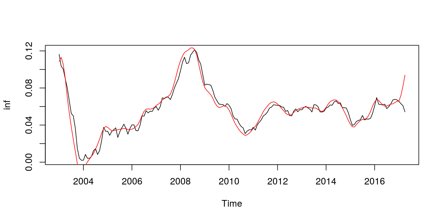

How Do You Filter In A Plot In R,
Source: https://kevinkotze.github.io/ts-5-tut/
Posted by: gurleygracts1948.blogspot.com
0 Response to "How Do You Filter In A Plot In R"
Post a Comment